R. Kyle Bocinsky, Timothy A. Kohler, Adam Brin, Keith W. Kintigh,
Bertram Ludäscher, Timothy McPhillips, Johnathan Rush
2016-02-05 (updated 2016-11-04)
The SKOPE Prototype is a Web application that provides reconstructed precipitation and temperature data at high spatial and temporal resolutions for the last 2000 years for the Four Corners region of the southwestern United States (Arizona, Colorado, New Mexico, and Utah) and portions of adjoining states. Using SKOPE, one can obtain estimates of the annual precipitation, growing season (May-September) precipitation, water year (October-September) precipitation, and growing season Fahrenheit growing degree days (GDD), for any period between 1 C.E. and 2000 C.E. for any 800m x 800m grid cell in the region.
Using the Tool
Navigate to the tool. Using a browser navigate to SKOPE prototype (SKOPE 2016). Reconstructed data are available for the green-shaded portion of the initial map display. The region in the extreme southwest near Tijuana, Mexico, is outside the study area (even though it is shaded green).
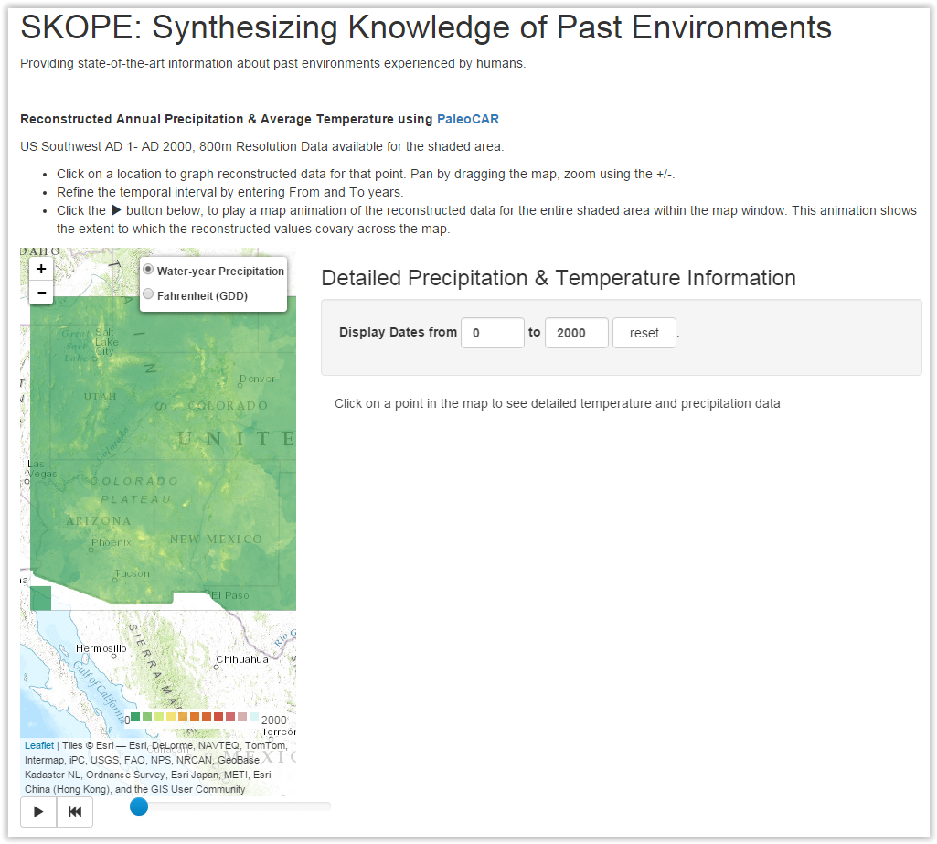
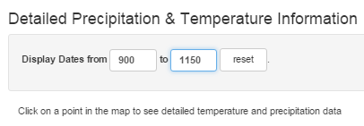
Identify the Time Period of Interest. To the right of the map, below where it says “Detailed Precipitation & Temperature Information”, is a box showing “Display Dates from 0 to 2000.” Replace the 0 with your starting year and replace the 2000 with your ending year, then click on a blank area in the prototype’s window. You can use the entire 1–2000 C.E. period but the prototype will operate faster and display more useful graphs with shorter intervals. To change the period at any point, simply enter different dates in the “from” and “to” boxes.
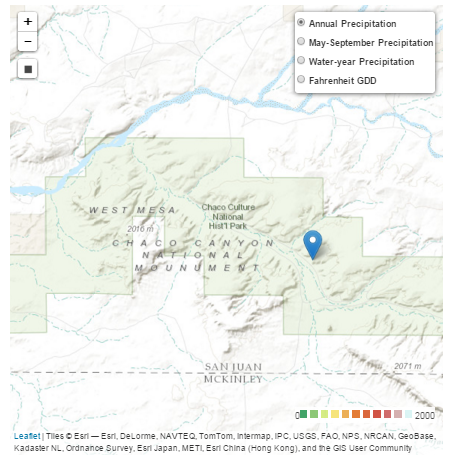
Drag the map and zoom in to display the area of interest. You can drag the map left and right and up and down by holding down the left mouse button and moving the mouse. You can zoom in using the + and – on the upper left corner of the map or by using a mouse scroll wheel. Multi-touch gestures on modern trackpads and touch-screens also work for zooming and scrolling.
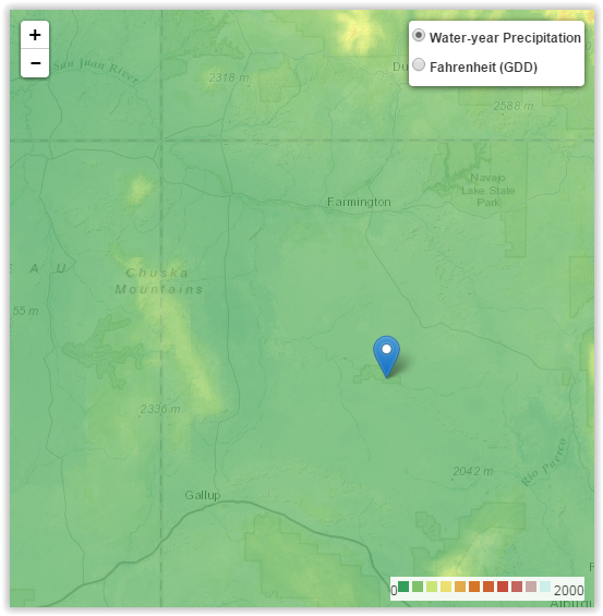
Select a Point of interest. Once you have zoomed in sufficiently to identify the specific area of interest, simply left click on the point and a blue flag will mark the spot.
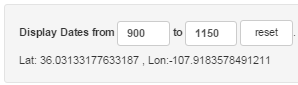
The precise longitude and latitude of the point you have selected are displayed below the date range.
Change the Point Focus. You can easily change the point focus by clicking on another spot. Each time you click a spot, the tool refreshes the data for the period and point of interest, so there will be a modest delay each time you change the point focus.
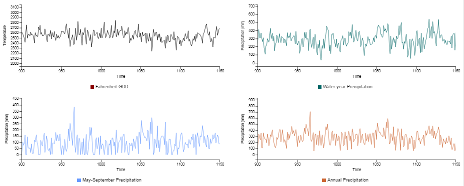
Examine Graphed Data for the Point. To the right of the map, graphs of the four climatic variables values are displayed, for the selected period of interest for your specific grid cell.
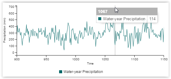
If you move the cursor into a given graph, you will see the year and climate value pop up for particular year corresponding to your cursor position.
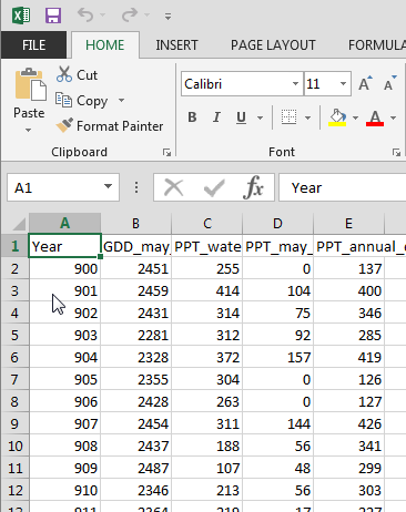
Download Point Data. If you are satisfied with your point and temporal interval selection, you can click on the Download Results button.

The vales of all four variables will be downloaded to your computer in a csv (comma separated value) file that can be opened by Excel. Just enter a folder location and file name (including the .csv extension), when prompted.
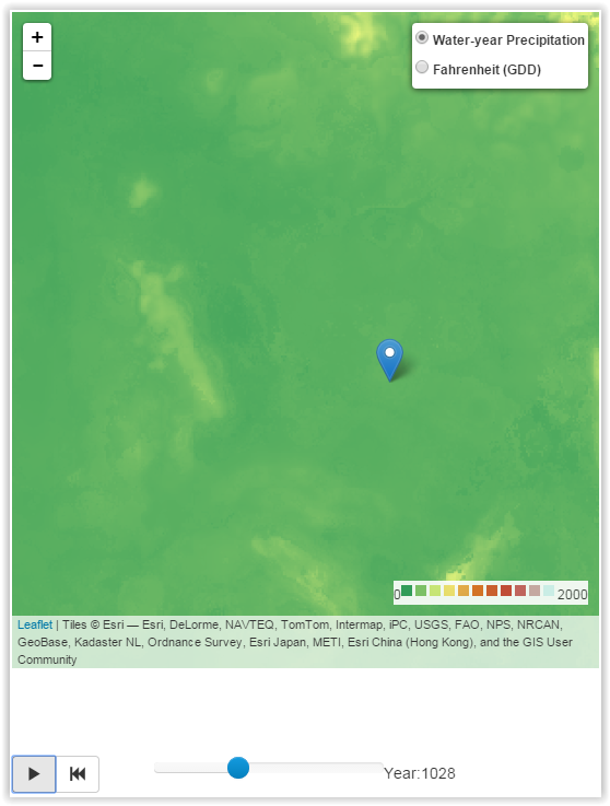
View Spatial Variation in a Retrodicted Variable over Time. In the upper right corner of the map, click on the radio button for the variable of interest. (At this point only Water-year Precipitation and Fahrenheit Growing Degree Days are implemented). Drag the map and zoom in or out and to display your area of interest.
Play an Animation. Click on the play button below the lower left corner of the map. The map display will cycle through your years of interest, with colors corresponding to the scale at the lower right corner of the map, for the selected variable. There may be a delay before the animation loads. You can hit the pause button to stop the animation or replay to start it again. The blue dot show the animations progress through the years, and you can click and hold the dot to move forward or backwards in time.
Methods
Paleoclimate reconstructions are created using the analytical package Paleoclimate Reconstruction from Tree Rings using Correlation-Adjusted coRrelation (PaleoCAR) which is developed in R, a free software environment for statistical computing (Bocinsky 2015). PaleoCAR relies on published tree-ring chronologies and PRISM’s spatially modeled historical climate signals to generate long-term reconstructions (Bocinsky and Kohler 2014; Bocinsky et al. in review). Tree ring chronologies were selected from the publically available International Tree Ring Data Bank (ITRDB; Grissino-Mayer 2015; and Fritts 1997) and were geographically limited to include only chronologies within a 10-degree buffer of the Four Corners states, including Arizona, New Mexico, Utah, and Colorado. ITRDB data were downloaded and processed using the FedData package in R (Bocinsky 2016). Historical climate signals were selected from PRISM’s spatially interpolated monthly 800m x 800m grid cells (which take into account elevation and several aspects of topography; PRISM Climate Group 2004; Daly et al. 2008). The historical calibration data set was limited to A.D. 1924–1983 (Bocinsky and Kohler 2014).
To generate the reconstruction, PaleoCAR utilizes the CAR (Correlation-Adjusted corRelation) variable ranking and selection method to identify grid-cell specific combinations of tree ring chronologies that best estimate PRISM’s historical (1924–1983) values for that cell. PaleoCAR uses the long-term tree ring chronologies to create reconstructions of precipitation and growing-degree days that extend back to 1 C.E. (see Bocinsky and Kohler 2014 for complete methodology; Bocinsky et al. 2016). The result is an ~800m (30 arc-second) resolution data grid of a 2,000 year (1–2000 C.E.) spatiotemporal paleoclimate reconstruction for each climate signal.
Caveats
Error. The retrodictions provided by this tool are, of course, estimates subject to error. There is some error in the spatial interpolation done by PRISM. There is also retrodiction model error that is dependent both on the location and the year, with earlier years generally having larger errors than more recent ones (when more tree ring chronologies can be referenced). In this version, we do not provide specific error estimates but see Bocinsky et al. (2016) for a discussion of the error.
Need for Spatial Smoothing. Each grid cell independently selects the best-fitting set of tree-ring chronologies to use in the retrodiction in a given year. However, because the selections are done independently, adjacent cells can pick different chronologies. A single difference in the chronologies selected can have a substantial impact on the retrodicted values, especially if the cell is in an area that has a weaker association between chronologies and the historic PRISM climate signal. This is more of problem with temperature than with precipitation, especially in lower-elevation areas. While future versions of the tool will provide the option of spatial smoothing to reduce the impact of these discontinuities, in current use it might be well to download point data for several spots within the area of interest. If there are substantial differences, the annual values should then be averaged.
Temporal Smoothing. The retrodicted data are not smoothed. For some analytical purposes, temporal smoothing of the downloaded data may be advisable (see Bocinsky et al. 2016).
References Cited
Bocinsky, R. Kyle. 2015. PaleoCAR: Paleoclimate Reconstruction from Tree Rings using Correlation Adjusted correlation. R package version 2.1. https://github.com/bocinsky/PaleoCAR/archive/2.1.tar.gz.
Bocinsky, R. Kyle. 2016. FedData: Functions to Automate Downloading Geospatial Data Available from Several Federated Data Sources. R package version 2.0.4.
http://CRAN.R-project.org/package=FedData
Bocinsky, R. Kyle, and Timothy A. Kohler. 2014. A 2,000-year reconstruction of the rain-fed maize agricultural niche in the US Southwest. Nature Communications 5:5618. DOI: 10.1038/ncomms6618
Bocinsky, R. Kyle, Johnathan Rush, Keith W. Kintigh, and Timothy A. Kohler. 2016. Exploration and exploitation in the macrohistory of the prehispanic Pueblo Southwest. Science Advances 2(4): e1501532 (01 Apr 2016) DOI: 10.1126/sciadv.1501532 http://advances.sciencemag.org/content/2/4/e1501532
Daly, Christopher, Michael Halbleib, Joseph I. Smith, Wayne P. Gibson, Matthew K. Doggett, George H. Taylor, Jan Curtis and Phillip P. Pasteris. 2008 Physiographically sensitive mapping of climatological temperature and precipitation across the conterminous United States. International Journal of Climatology. DOI: 10.1002/joc.1688
Grissino-Mayer, H.D. 2015 The International Tree Ring Data Bank. Accessed and available at http://web.utk.edu/~grissino/itrdb.htm .
Grissino-Mayer, Henri D. and Harold C. Fritts. 1997 The International Tree-Ring Data Bank: An enhanced global database serving the global scientific community, The Holocene 7: 235–238.
SKOPE. 2016 SKOPE Prototype. http://demo.envirecon.org/browse/ doi:10.6067/XCV8ZW1NM5